Loading IMPROVE Data
In this tutorial we will read and load data from the IMPROVE aerosol network (http://vista.cira.colostate.edu/Improve/)
To do this we need to first download the data from the colstate.edu website. There are a few format requirements needed to be compatible with MONET. First go to http://views.cira.colostate.edu/fed/DataWizard/Default.aspx to download data.
Select the Raw data
Datasets is the “IMPROVE aerosol”
Select any number of sites
Select your parameters
Select the dates in question
Fields
Dataset (required)
Site (required)
POC (required)
Date (required)
Parameter (required)
Data Value (required)
Latitude (required)
Longitude (required)
State (optional)
EPACode (optional)
Options
skinny format
delimited (note you will need to pass this onto the open command, ‘,’ by default)
After downloading we can then read the data. Here we included the EPACode and State to add additional meta data stored on the EPA auxiliary files used in the EPA AQS and AirNow datasets in MONET. Let’s make a few imports from monet and some other libraries that will aid us later.
from monet.obs import improve
import matplotlib.pyplot as plt
from monet.util import tools
from monet.plots import *
import pandas as pd
Now we will load the data (in this case the file is ‘2018620155016911Q1N0Mq.txt’)
df = improve.add_data('/Users/barry/Desktop/20186258419212M0xuxu.txt', add_meta=False, delimiter=',')
from numpy import NaN
df['obs'].loc[df.obs < 0] = NaN
/anaconda3/lib/python3.6/site-packages/pandas/core/indexing.py:189: SettingWithCopyWarning:
A value is trying to be set on a copy of a slice from a DataFrame

See the caveats in the documentation: http://pandas.pydata.org/pandas-docs/stable/indexing.html#indexing-view-versus-copy
  self._setitem_with_indexer(indexer, value)
Let’s look at the dataframe.
df.head(20)
| siteid | poc | time | variable | obs | unc | mdl | units | latitude | longitude | elevation | state_name | epaid | |
|---|---|---|---|---|---|---|---|---|---|---|---|---|---|
| 0 | ACAD1 | 1 | 2016-01-01 | ALf | NaN | 0.00121 | 0.00199 | ug/m^3 LC | 44.3771 | -68.261 | 157.3333 | ME | 230090103 |
| 1 | ACAD1 | 1 | 2016-01-01 | ASf | NaN | 0.00014 | 0.00022 | ug/m^3 LC | 44.3771 | -68.261 | 157.3333 | ME | 230090103 |
| 2 | ACAD1 | 1 | 2016-01-01 | BRf | 0.00050 | 0.00011 | 0.00016 | ug/m^3 LC | 44.3771 | -68.261 | 157.3333 | ME | 230090103 |
| 3 | ACAD1 | 1 | 2016-01-01 | CAf | NaN | 0.00143 | 0.00234 | ug/m^3 LC | 44.3771 | -68.261 | 157.3333 | ME | 230090103 |
| 4 | ACAD1 | 1 | 2016-01-01 | CHLf | NaN | 0.00376 | 0.00744 | ug/m^3 LC | 44.3771 | -68.261 | 157.3333 | ME | 230090103 |
| 5 | ACAD1 | 1 | 2016-01-01 | CLf | 0.00085 | 0.00051 | 0.00081 | ug/m^3 LC | 44.3771 | -68.261 | 157.3333 | ME | 230090103 |
| 6 | ACAD1 | 1 | 2016-01-01 | CRf | 0.00015 | 0.00010 | 0.00015 | ug/m^3 LC | 44.3771 | -68.261 | 157.3333 | ME | 230090103 |
| 7 | ACAD1 | 1 | 2016-01-01 | CUf | NaN | 0.00014 | 0.00022 | ug/m^3 LC | 44.3771 | -68.261 | 157.3333 | ME | 230090103 |
| 8 | ACAD1 | 1 | 2016-01-01 | ECf | 0.11758 | 0.01481 | 0.00900 | ug/m^3 LC | 44.3771 | -68.261 | 157.3333 | ME | 230090103 |
| 9 | ACAD1 | 1 | 2016-01-01 | EC1f | 0.15773 | 0.01700 | 0.01270 | ug/m^3 LC | 44.3771 | -68.261 | 157.3333 | ME | 230090103 |
| 10 | ACAD1 | 1 | 2016-01-01 | EC2f | 0.08037 | 0.01439 | 0.00900 | ug/m^3 LC | 44.3771 | -68.261 | 157.3333 | ME | 230090103 |
| 11 | ACAD1 | 1 | 2016-01-01 | EC3f | NaN | 0.00450 | 0.00900 | ug/m^3 LC | 44.3771 | -68.261 | 157.3333 | ME | 230090103 |
| 12 | ACAD1 | 1 | 2016-01-01 | FEf | 0.00397 | 0.00088 | 0.00139 | ug/m^3 LC | 44.3771 | -68.261 | 157.3333 | ME | 230090103 |
| 13 | ACAD1 | 1 | 2016-01-01 | Kf | 0.01480 | 0.00069 | 0.00087 | ug/m^3 LC | 44.3771 | -68.261 | 157.3333 | ME | 230090103 |
| 14 | ACAD1 | 1 | 2016-01-01 | MF | 1.38909 | 0.16326 | 0.31570 | ug/m^3 LC | 44.3771 | -68.261 | 157.3333 | ME | 230090103 |
| 15 | ACAD1 | 1 | 2016-01-01 | MGf | NaN | 0.00207 | 0.00340 | ug/m^3 LC | 44.3771 | -68.261 | 157.3333 | ME | 230090103 |
| 16 | ACAD1 | 1 | 2016-01-01 | MNf | NaN | 0.00020 | 0.00033 | ug/m^3 LC | 44.3771 | -68.261 | 157.3333 | ME | 230090103 |
| 17 | ACAD1 | 1 | 2016-01-01 | MT | 2.80114 | 0.22824 | 0.42441 | ug/m^3 LC | 44.3771 | -68.261 | 157.3333 | ME | 230090103 |
| 18 | ACAD1 | 1 | 2016-01-01 | N2f | NaN | 0.02791 | 0.05438 | ug/m^3 LC | 44.3771 | -68.261 | 157.3333 | ME | 230090103 |
| 19 | ACAD1 | 1 | 2016-01-01 | NAf | NaN | 0.00257 | 0.00412 | ug/m^3 LC | 44.3771 | -68.261 | 157.3333 | ME | 230090103 |
Now this is in the long pandas format. Let’s use the
monet.util.tools.long_to_wide utility to reformat the dataframe into a
wide format.
from monet.util import tools
df1 = tools.long_to_wide(df)
df1.head()
| time | siteid | ALf | ASf | BRf | CAf | CHLf | CLf | CM_calculated | CRf | ... | variable | obs | unc | mdl | units | latitude | longitude | elevation | state_name | epaid | |
|---|---|---|---|---|---|---|---|---|---|---|---|---|---|---|---|---|---|---|---|---|---|
| 0 | 2016-01-01 | ACAD1 | NaN | NaN | 0.0005 | NaN | NaN | 0.00085 | 1.41205 | 0.00015 | ... | ALf | NaN | 0.00121 | 0.00199 | ug/m^3 LC | 44.3771 | -68.261 | 157.3333 | ME | 230090103 |
| 1 | 2016-01-01 | ACAD1 | NaN | NaN | 0.0005 | NaN | NaN | 0.00085 | 1.41205 | 0.00015 | ... | ASf | NaN | 0.00014 | 0.00022 | ug/m^3 LC | 44.3771 | -68.261 | 157.3333 | ME | 230090103 |
| 2 | 2016-01-01 | ACAD1 | NaN | NaN | 0.0005 | NaN | NaN | 0.00085 | 1.41205 | 0.00015 | ... | BRf | 0.0005 | 0.00011 | 0.00016 | ug/m^3 LC | 44.3771 | -68.261 | 157.3333 | ME | 230090103 |
| 3 | 2016-01-01 | ACAD1 | NaN | NaN | 0.0005 | NaN | NaN | 0.00085 | 1.41205 | 0.00015 | ... | CAf | NaN | 0.00143 | 0.00234 | ug/m^3 LC | 44.3771 | -68.261 | 157.3333 | ME | 230090103 |
| 4 | 2016-01-01 | ACAD1 | NaN | NaN | 0.0005 | NaN | NaN | 0.00085 | 1.41205 | 0.00015 | ... | CHLf | NaN | 0.00376 | 0.00744 | ug/m^3 LC | 44.3771 | -68.261 | 157.3333 | ME | 230090103 |
5 rows × 65 columns
Let’s now plot some of the different measurements with time from a site. In this case we will look at the PHOE1 site in Phoenix, Arizona.
acad1 = df1.loc[df1.siteid == 'ACAD1']
acad1.head()
| time | siteid | ALf | ASf | BRf | CAf | CHLf | CLf | CM_calculated | CRf | ... | variable | obs | unc | mdl | units | latitude | longitude | elevation | state_name | epaid | |
|---|---|---|---|---|---|---|---|---|---|---|---|---|---|---|---|---|---|---|---|---|---|
| 0 | 2016-01-01 | ACAD1 | NaN | NaN | 0.0005 | NaN | NaN | 0.00085 | 1.41205 | 0.00015 | ... | ALf | NaN | 0.00121 | 0.00199 | ug/m^3 LC | 44.3771 | -68.261 | 157.3333 | ME | 230090103 |
| 1 | 2016-01-01 | ACAD1 | NaN | NaN | 0.0005 | NaN | NaN | 0.00085 | 1.41205 | 0.00015 | ... | ASf | NaN | 0.00014 | 0.00022 | ug/m^3 LC | 44.3771 | -68.261 | 157.3333 | ME | 230090103 |
| 2 | 2016-01-01 | ACAD1 | NaN | NaN | 0.0005 | NaN | NaN | 0.00085 | 1.41205 | 0.00015 | ... | BRf | 0.0005 | 0.00011 | 0.00016 | ug/m^3 LC | 44.3771 | -68.261 | 157.3333 | ME | 230090103 |
| 3 | 2016-01-01 | ACAD1 | NaN | NaN | 0.0005 | NaN | NaN | 0.00085 | 1.41205 | 0.00015 | ... | CAf | NaN | 0.00143 | 0.00234 | ug/m^3 LC | 44.3771 | -68.261 | 157.3333 | ME | 230090103 |
| 4 | 2016-01-01 | ACAD1 | NaN | NaN | 0.0005 | NaN | NaN | 0.00085 | 1.41205 | 0.00015 | ... | CHLf | NaN | 0.00376 | 0.00744 | ug/m^3 LC | 44.3771 | -68.261 | 157.3333 | ME | 230090103 |
5 rows × 65 columns
Trend Analysis
Let’s look at SIf as an example from ACAD1.
acad1.index = acad1.time

acad1.plot(y='SIf', figsize=(14,5))
<matplotlib.axes._subplots.AxesSubplot at 0x1c286eb4a8>
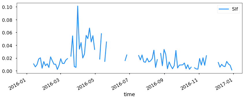
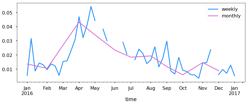
Now this is good, but let’s resample to see if we can see a trend.
ax = acad1.resample('W').mean().plot(y='SIf', figsize=(14,5), label = 'weekly')
ax = acad1.resample('M').mean().plot(y='SIf', ax=ax, label='monthly')
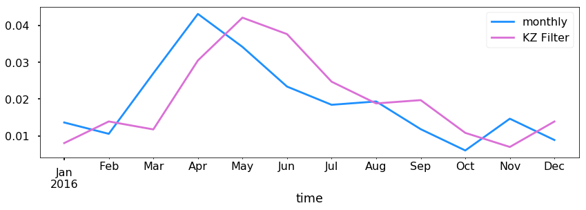
Simply resampling is fine, but let’s try to get a signal out using a Kolmogorov–Zurbenko filter. See https://doi.org/10.1080/10473289.2005.10464718 for more information.
q = acad1.SIf.copy()
for i in range(1000):
    q = q.rolling(10, min_periods=1, win_type='triang',center=True).mean()
ax = acad1.resample('M').mean().plot(y='SIf', figsize=(14,4), label='monthly')
q.resample('M').mean().plot(ax=ax,label='KZ Filter')
plt.legend()
<matplotlib.legend.Legend at 0x1c290de080>
KMEANS Clustering using scikit-learn
Clustering algorithms can be very useful in finding signals within data. As an example we are going to use the KMeans algorithm from scikit-learn (http://scikit-learn.org/stable/modules/clustering.html#k-means) to analyse dust signals using the improve data. First we need to import some tools from sklearn to use in our analysis.
from sklearn.preprocessing import RobustScaler # to scale our data
from sklearn.cluster import KMeans # clustering algorithm
First we want to separate out different variables that may be useful such as Si, PM2.5, PM10, Fe, and SOILf. We will also need to drop any NaN values so let us go ahead and do that.
dfkm = df1[['SIf','MF','MT','FEf','SOILf']].dropna()
dfkm.head()
| SIf | MF | MT | FEf | SOILf | |
|---|---|---|---|---|---|
| 0 | 0.00553 | 1.38909 | 2.80114 | 0.00397 | 0.028611 |
| 1 | 0.00553 | 1.38909 | 2.80114 | 0.00397 | 0.028611 |
| 2 | 0.00553 | 1.38909 | 2.80114 | 0.00397 | 0.028611 |
| 3 | 0.00553 | 1.38909 | 2.80114 | 0.00397 | 0.028611 |
| 4 | 0.00553 | 1.38909 | 2.80114 | 0.00397 | 0.028611 |
Usually, with sklearn it is better to scale the data first before putting it through the algorithm. We will use the RobustScaler to do this.
X_scaled = RobustScaler().fit(dfkm).transform(dfkm)
Now we will define our clustering algorithm to have 2 clusters. You may need to adjust this as this is just a starting point for further analysis.
km = KMeans(n_clusters=2).fit(X_scaled)
The clusters can be found under km.labels_. These are integers
representing the different clusters.
clusters = km.labels_
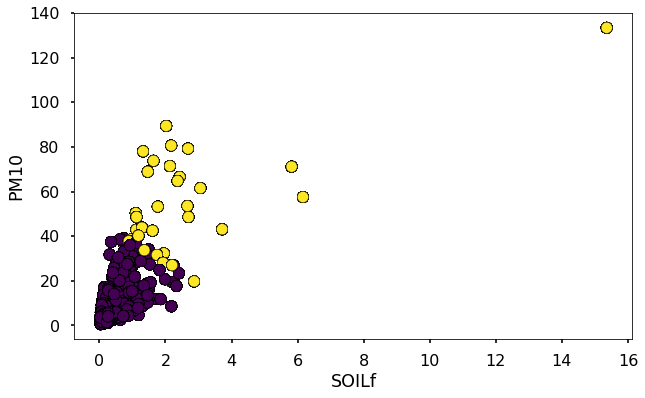
Let’s plot this so that we can see where there is dust.
plt.figure(figsize=(10,6))
plt.scatter(dfkm.SOILf,dfkm.MT,c=clusters,edgecolor='k')
plt.xlabel('SOILf')
plt.ylabel('PM10')
Text(0,0.5,'PM10')