How to read AQS data from PAMS and do a quick analysis
The first tutorial for MONET will load data from the AQS data, specifically the PAMS dataset, and show to reshape the dataframe and do a statistical analysis with different meteorological and composition data. For more examples, please see https://monet-arl.readthedocs.io/en/develop/. This will later be able to be found on the github page and readthedocs.
We will first begin by importing monet and a few helper classes for later
import numpy as np          # numpy
import pandas as pd         # pandas
import monetio as mio       # observations from MONET
import matplotlib.pyplot as plt # plotting
import seaborn as sns       # better color palettes
import cartopy.crs as ccrs  # map projections
import cartopy.feature as cfeature # politcal and geographic features
sns.set_style('ticks')   # plot configuration
sns.set_context("talk")  # plot configure for size of text
Now we have all the imports we could need lets load some data. Most of the PAMS data is on daily data so lets add the kwarg daily=True to the call. We will also create this for the year 2015 and 2016. Some variables that may be valuable are the VOCS, ozone, NO2, NOX, temperature. For all of the measurements available please see https://aqs.epa.gov/aqsweb/airdata/download_files.html
dates = pd.date_range(start='2004-01-01',end='2004-12-31')
df = mio.aqs.add_data(dates,daily=True,param=['VOC','OZONE'], download=True)
 Retrieving: daily_VOCS_2004.zip
https://aqs.epa.gov/aqsweb/airdata/daily_VOCS_2004.zip


 Retrieving: daily_44201_2004.zip
https://aqs.epa.gov/aqsweb/airdata/daily_44201_2004.zip


[########################################] | 100% Completed | 26.1s
[########################################] | 100% Completed | 26.2s
[########################################] | 100% Completed | 26.3s
[########################################] | 100% Completed | 26.4s
[########################################] | 100% Completed | 26.5s
[########################################] | 100% Completed | 34.8s
[########################################] | 100% Completed | 34.9s
[########################################] | 100% Completed | 34.9s
[########################################] | 100% Completed | 35.0s
[########################################] | 100% Completed | 35.1s
Monitor File Path: /anaconda3/lib/python3.6/site-packages/data/monitoring_site_locations.hdf
Monitor File Not Found... Reprocessing
/anaconda3/lib/python3.6/site-packages/python/core/interactiveshell.py:2963: DtypeWarning: Columns (0) have mixed types. Specify dtype option on import or set low_memory=False.
  exec(code_obj, self.user_global_ns, self.user_ns)
/anaconda3/lib/python3.6/site-packages/pandas/core/indexing.py:189: SettingWithCopyWarning:
A value is trying to be set on a copy of a slice from a DataFrame

See the caveats in the documentation: http://pandas.pydata.org/pandas-docs/stable/indexing.html#indexing-view-versus-copy
  self._setitem_with_indexer(indexer, value)
Now we have the data in aqs.df and a copy of it in df… just in case. So lets take a look at it.
#df.head()
df.head()
| time_local | state_code | county_code | site_num | parameter_code | poc | latitude | longitude | datum | parameter_name | ... | first_year_of_data | gmt_offset | land_use | location_setting | monitor_type | msa_code | networks | state_name | tribe_name | time | |
|---|---|---|---|---|---|---|---|---|---|---|---|---|---|---|---|---|---|---|---|---|---|
| 0 | 2004-05-15 | 04 | 013 | 4003 | 43000 | 10 | 33.40316 | -112.07533 | WGS84 | Sum of PAMS target compounds | ... | NaN | -7.0 | RESIDENTIAL | URBAN AND CENTER CITY | OTHER | NaN | NaN | AZ | NaN | 2004-05-15 07:00:00 |
| 1 | 2004-05-21 | 04 | 013 | 4003 | 43000 | 10 | 33.40316 | -112.07533 | WGS84 | Sum of PAMS target compounds | ... | NaN | -7.0 | RESIDENTIAL | URBAN AND CENTER CITY | OTHER | NaN | NaN | AZ | NaN | 2004-05-21 07:00:00 |
| 2 | 2004-05-27 | 04 | 013 | 4003 | 43000 | 10 | 33.40316 | -112.07533 | WGS84 | Sum of PAMS target compounds | ... | NaN | -7.0 | RESIDENTIAL | URBAN AND CENTER CITY | OTHER | NaN | NaN | AZ | NaN | 2004-05-27 07:00:00 |
| 3 | 2004-06-02 | 04 | 013 | 4003 | 43000 | 10 | 33.40316 | -112.07533 | WGS84 | Sum of PAMS target compounds | ... | NaN | -7.0 | RESIDENTIAL | URBAN AND CENTER CITY | OTHER | NaN | NaN | AZ | NaN | 2004-06-02 07:00:00 |
| 4 | 2004-06-08 | 04 | 013 | 4003 | 43000 | 10 | 33.40316 | -112.07533 | WGS84 | Sum of PAMS target compounds | ... | NaN | -7.0 | RESIDENTIAL | URBAN AND CENTER CITY | OTHER | NaN | NaN | AZ | NaN | 2004-06-08 07:00:00 |
5 rows × 46 columns
Notice that in this printed format it obscures some of the dataframe columns from view. Lets see what they are!
from numpy import sort
for i in sort(df.columns): # loop over the sorted columns and print them
    print(i)
1st_max_hour
1st_max_value
address
airnow_flag
aqi
cbsa_name
city_name
cmsa_name
collecting_agency
county_code
county_name
date_of_last_change
datum
elevation
epa_region
event_type
first_year_of_data
gmt_offset
land_use
latitude
local_site_name
location_setting
longitude
method_code
method_name
monitor_type
msa_code
msa_name
networks
obs
observation_count
observation_percent
parameter_code
parameter_name
poc
pollutant_standard
sample_duration
site_num
siteid
state_code
state_name
time
time_local
tribe_name
units
variable
We have lots of columns but this is actually the long format (data is stacked on variable). Data analysis could be done easier in a wide format. So lets use a utility function in MONET to aid with reshaping the dataframe.
from monet.util import tools
new = tools.long_to_wide(df)
new.head()
| time | siteid | 1,1,2,2-TETRACHLOROETHANE | 1,1,2-TRICHLORO-1,2,2-TRIFLUOROETHANE | 1,1,2-TRICHLOROETHANE | 1,1-DICHLOROETHANE | 1,1-DICHLOROETHYLENE | 1,2,3-TRIMETHYLBENZENE | 1,2,4-TRICHLOROBENZENE | 1,2,4-TRIMETHYLBENZENE | ... | epa_region | first_year_of_data | gmt_offset | land_use | location_setting | monitor_type | msa_code | networks | state_name | tribe_name | |
|---|---|---|---|---|---|---|---|---|---|---|---|---|---|---|---|---|---|---|---|---|---|
| 0 | 2004-01-01 05:00:00 | 090031003 | NaN | NaN | NaN | NaN | NaN | NaN | NaN | NaN | ... | NaN | 2002.0 | -5.0 | RESIDENTIAL | SUBURBAN | NaN | NaN | NaN | CT | NaN |
| 1 | 2004-01-01 05:00:00 | 100031007 | NaN | NaN | NaN | NaN | NaN | NaN | NaN | NaN | ... | NaN | 2003.0 | -5.0 | AGRICULTURAL | RURAL | OTHER | NaN | NaN | DE | NaN |
| 2 | 2004-01-01 05:00:00 | 100031013 | NaN | NaN | NaN | NaN | NaN | NaN | NaN | NaN | ... | NaN | 2003.0 | -5.0 | RESIDENTIAL | SUBURBAN | SLAMS | NaN | NaN | DE | NaN |
| 3 | 2004-01-01 05:00:00 | 110010025 | NaN | NaN | NaN | NaN | NaN | NaN | NaN | NaN | ... | NaN | 1980.0 | -5.0 | COMMERCIAL | URBAN AND CENTER CITY | NaN | NaN | NaN | District Of Columbia | NaN |
| 4 | 2004-01-01 05:00:00 | 110010041 | NaN | NaN | NaN | NaN | NaN | NaN | NaN | NaN | ... | NaN | 1993.0 | -5.0 | RESIDENTIAL | URBAN AND CENTER CITY | NaN | NaN | NaN | District Of Columbia | NaN |
5 rows × 157 columns
Lets see how many ISOPRENE sites there are. We will drop the NaN values along the ISOPRENE column and then find the unique siteid’s and look at the shape of them
new.dropna(subset=['ISOPRENE']).siteid.unique().shape
(140,)
Now as you can see we have lots of columns that is sorted by time and siteid. But what measurements are included in the dataframe? Let’s see all the new columns generated from pivoting the table.
from numpy import sort
for i in sort(new.columns):
    print(i)
1,1,2,2-TETRACHLOROETHANE
1,1,2-TRICHLORO-1,2,2-TRIFLUOROETHANE
1,1,2-TRICHLOROETHANE
1,1-DICHLOROETHANE
1,1-DICHLOROETHYLENE
1,2,3-TRIMETHYLBENZENE
1,2,4-TRICHLOROBENZENE
1,2,4-TRIMETHYLBENZENE
1,2-DICHLOROBENZENE
1,2-DICHLOROPROPANE
1,3,5-TRIMETHYLBENZENE
1,3-BUTADIENE
1,3-DICHLOROBENZENE
1,4-DICHLOROBENZENE
1-BUTENE
1-PENTENE
1st_max_hour
1st_max_value
2,2,4-TRIMETHYLPENTANE
2,2-DIMETHYLBUTANE
2,3,4-TRIMETHYLPENTANE
2,3-DIMETHYLBUTANE
2,3-DIMETHYLPENTANE
2,4-DIMETHYLPENTANE
2-METHYLHEPTANE
2-METHYLHEXANE
2-METHYLPENTANE
3-CHLOROPROPENE
3-METHYLHEPTANE
3-METHYLHEXANE
3-METHYLPENTANE
ACETALDEHYDE
ACETONE
ACETONITRILE
ACETYLENE
ACROLEIN - UNVERIFIED
ACRYLONITRILE
BENZENE
BENZYL CHLORIDE
BROMOCHLOROMETHANE
BROMODICHLOROMETHANE
BROMOFORM
BROMOMETHANE
CARBON DISULFIDE
CARBON TETRACHLORIDE
CHLOROBENZENE
CHLOROETHANE
CHLOROFORM
CHLOROMETHANE
CHLOROPRENE
CIS-1,2-DICHLOROETHENE
CIS-1,3-DICHLOROPROPENE
CIS-2-BUTENE
CIS-2-PENTENE
CYCLOHEXANE
CYCLOPENTANE
DIBROMOCHLOROMETHANE
DICHLORODIFLUOROMETHANE
DICHLOROMETHANE
ETHANE
ETHYL ACRYLATE
ETHYLBENZENE
ETHYLENE
ETHYLENE DIBROMIDE
ETHYLENE DICHLORIDE
FORMALDEHYDE
FREON 113
FREON 114
HEXACHLOROBUTADIENE
ISOBUTANE
ISOPENTANE
ISOPRENE
ISOPROPYLBENZENE
M-DIETHYLBENZENE
M-ETHYLTOLUENE
M/P XYLENE
METHYL CHLOROFORM
METHYL ETHYL KETONE
METHYL ISOBUTYL KETONE
METHYL METHACRYLATE
METHYL TERT-BUTYL ETHER
METHYLCYCLOHEXANE
METHYLCYCLOPENTANE
N-BUTANE
N-DECANE
N-HEPTANE
N-HEXANE
N-NONANE
N-OCTANE
N-PENTANE
N-PROPYLBENZENE
N-UNDECANE
O-ETHYLTOLUENE
O-XYLENE
OZONE
P-DIETHYLBENZENE
P-ETHYLTOLUENE
PROPANE
PROPYLENE
STYRENE
SUM OF PAMS TARGET COMPOUNDS
TERT-AMYL METHYL ETHER
TERT-BUTYL ETHYL ETHER
TETRACHLOROETHYLENE
TOLUENE
TOTAL NMOC (NON-METHANE ORGANIC COMPOUND)
TRANS-1,2-DICHLOROETHYLENE
TRANS-1,3-DICHLOROPROPENE
TRANS-2-BUTENE
TRANS-2-PENTENE
TRICHLOROETHYLENE
TRICHLOROFLUOROMETHANE
VINYL CHLORIDE
address
airnow_flag
aqi
cbsa_name
city_name
cmsa_name
collecting_agency
county_code
county_name
date_of_last_change
datum
elevation
epa_region
event_type
first_year_of_data
gmt_offset
land_use
latitude
local_site_name
location_setting
longitude
method_code
method_name
monitor_type
msa_code
msa_name
networks
obs
observation_count
observation_percent
parameter_code
parameter_name
poc
pollutant_standard
sample_duration
site_num
siteid
state_code
state_name
time
time_local
tribe_name
units
variable
Now as you can see we have lots of columns that is sorted by time and siteid. This can be very useful as we can now do some direct comparisons using the dataframe. Lets get a description of the dataset first so we can see some averages and ranges of the different chemical species.
new.describe()
| 1,1,2,2-TETRACHLOROETHANE | 1,1,2-TRICHLORO-1,2,2-TRIFLUOROETHANE | 1,1,2-TRICHLOROETHANE | 1,1-DICHLOROETHANE | 1,1-DICHLOROETHYLENE | 1,2,3-TRIMETHYLBENZENE | 1,2,4-TRICHLOROBENZENE | 1,2,4-TRIMETHYLBENZENE | 1,2-DICHLOROBENZENE | 1,2-DICHLOROPROPANE | ... | obs | 1st_max_value | 1st_max_hour | aqi | method_code | cmsa_name | elevation | first_year_of_data | gmt_offset | msa_code | |
|---|---|---|---|---|---|---|---|---|---|---|---|---|---|---|---|---|---|---|---|---|---|
| count | 714352.000000 | 132606.000000 | 665982.000000 | 475211.000000 | 704962.000000 | 766240.000000 | 407466.000000 | 1.105874e+06 | 441391.000000 | 713931.000000 | ... | 1.501618e+06 | 1.501618e+06 | 1.501618e+06 | 335758.000000 | 1.165860e+06 | 0.0 | 0.0 | 1.393782e+06 | 1.501618e+06 | 0.0 |
| mean | 0.020421 | 0.169611 | 0.019323 | 0.012979 | 0.020375 | 0.474538 | 0.111623 | 1.011792e+00 | 0.129964 | 0.030783 | ... | 3.764996e+00 | 8.070852e+00 | 5.336468e+00 | 37.632730 | 1.404985e+02 | NaN | NaN | 1.993263e+03 | -5.978275e+00 | NaN |
| std | 0.157866 | 0.215456 | 0.158109 | 0.185480 | 0.178133 | 1.307923 | 1.129665 | 2.255642e+00 | 0.947958 | 0.230669 | ... | 3.997054e+01 | 1.091979e+02 | 6.966935e+00 | 19.249021 | 2.685583e+01 | NaN | NaN | 1.223728e+01 | 1.006215e+00 | NaN |
| min | 0.000000 | 0.000000 | 0.000000 | 0.000000 | 0.000000 | 0.000000 | 0.000000 | 0.000000e+00 | 0.000000 | 0.000000 | ... | 0.000000e+00 | 0.000000e+00 | 0.000000e+00 | 0.000000 | 1.100000e+01 | NaN | NaN | 1.959000e+03 | -1.000000e+01 | NaN |
| 25% | 0.000000 | 0.100000 | 0.000000 | 0.000000 | 0.000000 | 0.050000 | 0.000000 | 1.800000e-01 | 0.000000 | 0.000000 | ... | 2.000000e-02 | 3.000000e-02 | 0.000000e+00 | 26.000000 | 1.260000e+02 | NaN | NaN | 1.982000e+03 | -6.000000e+00 | NaN |
| 50% | 0.000000 | 0.180000 | 0.000000 | 0.000000 | 0.000000 | 0.230000 | 0.000000 | 5.000000e-01 | 0.000000 | 0.000000 | ... | 8.000000e-02 | 1.000000e-01 | 0.000000e+00 | 35.000000 | 1.280000e+02 | NaN | NaN | 1.997000e+03 | -6.000000e+00 | NaN |
| 75% | 0.010000 | 0.220000 | 0.010000 | 0.000000 | 0.010000 | 0.468182 | 0.000000 | 1.219583e+00 | 0.000000 | 0.020000 | ... | 6.600000e-01 | 1.000000e+00 | 1.000000e+01 | 43.000000 | 1.740000e+02 | NaN | NaN | 2.003000e+03 | -5.000000e+00 | NaN |
| max | 10.000000 | 10.000000 | 10.000000 | 10.000000 | 10.000000 | 39.266667 | 54.700000 | 1.493500e+02 | 59.880000 | 15.000000 | ... | 9.474708e+03 | 3.854257e+04 | 2.300000e+01 | 212.000000 | 2.110000e+02 | NaN | NaN | 2.018000e+03 | -4.000000e+00 | NaN |
8 rows × 127 columns
This gives us a format that allows simple statistics and plots using pandas, matplotlib, and seaborn. For time series it is often useful to have the index as the time. Lets do that
new.index = new.time
new['OZONE_ppb'] = new.OZONE * 1000.
new.OZONE_ppb.mean()
27.581303457170307
Plotting
As you can see the data is now indexed with the UTC time. Lets make a time series plot of the average ISOPRENE.
f,ax = plt.subplots(figsize=(10,4)) # this is so we can control the figure size.
new.ISOPRENE.resample('D').mean().plot(ax=ax)
<matplotlib.axes._subplots.AxesSubplot at 0x1c2bb1f860>
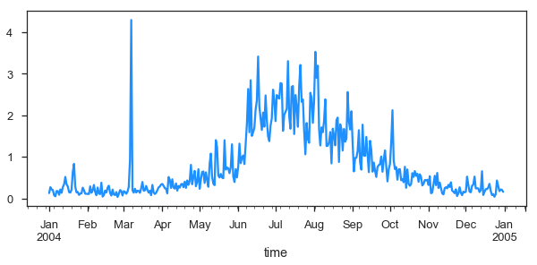
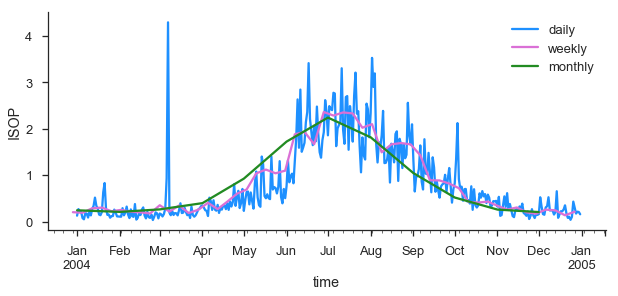
This is quite noisy with the daily data. Lets resample in time to every month using the average Isoprene concentration to weekly and monthly.
f,ax = plt.subplots(figsize=(10,4)) # this is so we can control the figure size.
new.ISOPRENE.resample('D').mean().plot(ax=ax, label='daily')
new.ISOPRENE.resample('W').mean().plot(ax=ax, label='weekly')
new.ISOPRENE.resample('M').mean().plot(ax=ax, label='monthly')
plt.ylabel('ISOP')
plt.legend()
sns.despine()
Where are these measurements. Lets plot this on a map and see where it is. We can use a utility plotting function in monet to generate the plot
from monet import plots
ax = plots.draw_map(states=True, extent=[-130,-60,20,50], resolution='10m')
# get only where ISOPRENE is not NAN
isop = new.dropna(subset=['ISOPRENE'])
ax.scatter(isop.longitude, isop.latitude)
<matplotlib.collections.PathCollection at 0x1c47460f60>
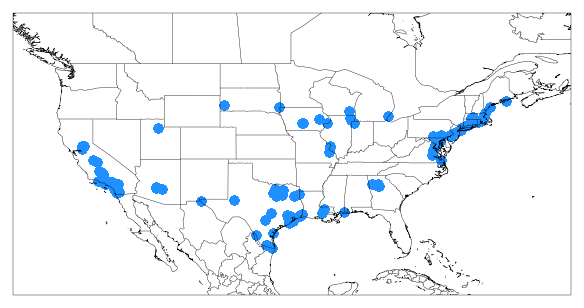
There are monitors all across the US with many in TX, CA, New England and the Mid-Atlantic.
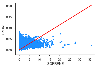
What if we wanted to do a linear regression between two variables. Lets say OZONE and temperature. To do this we will use the statsmodels package. It is a robust library for curve fitting. For specific information for this module look here https://www.statsmodels.org/stable/index.html
import statsmodels.api as sm # load statsmodels api
#first clean of nan values
fit_df = new[['ISOPRENE','OZONE']].dropna()
x = fit_df.ISOPRENE
y = fit_df.OZONE
result = sm.OLS(y,x).fit()
print(result.summary())

fit_df.plot.scatter(x='ISOPRENE',y='OZONE')
plt.plot(x,result.predict(x),'--r')
                            OLS Regression Results
==============================================================================
Dep. Variable:                  OZONE   R-squared:                       0.248
Model:                            OLS   Adj. R-squared:                  0.248
Method:                 Least Squares   F-statistic:                 1.833e+05
Date:                Tue, 19 Jun 2018   Prob (F-statistic):               0.00
Time:                        09:31:12   Log-Likelihood:             1.2390e+06
No. Observations:              556733   AIC:                        -2.478e+06
Df Residuals:                  556732   BIC:                        -2.478e+06
Df Model:                           1
Covariance Type:            nonrobust
==============================================================================
                 coef    std err          t      P>|t|      [0.025      0.975]
------------------------------------------------------------------------------
ISOPRENE       0.0057   1.33e-05    428.134      0.000       0.006       0.006
==============================================================================
Omnibus:                   205153.426   Durbin-Watson:                   0.007
Prob(Omnibus):                  0.000   Jarque-Bera (JB):          2465877.353
Skew:                          -1.433   Prob(JB):                         0.00
Kurtosis:                      12.904   Cond. No.                         1.00
==============================================================================

Warnings:
[1] Standard Errors assume that the covariance matrix of the errors is correctly specified.
[<matplotlib.lines.Line2D at 0x1c1e7f0f28>]
Lets save this to a csv file
new.to_csv('/Users/barry/Desktop/new.csv')