FV3-CHEM in MONET
FV3-CHEM is the experimental implementation of the NASA Gocart model into NOAA’s Next Generation Global Prediction System. This tutorial will explain how to open read and use MONET to explore output from the FV3-CHEM system.
Currently, FV3 outputs data in three formats, i.e., nemsio, grib2, and netcdf. There are slight issues with both the nemsio and grib2 data that will be explained below but needless to say they need to be converted with precossors.
Convert nemsio2nc4
The first format that needs to be converted is the nemsio data. NOTE: The nemsio format will be discontinued as of GFSv16. This step will not be needed to read the output data. nemsio is a binary format used within EMC for GFSv15 and previous versions. As a work around a converter was created to convert the binary nemsio data into netCDF, nemsio2nc4.py.
This is a command-line script that converts the nemsio data output by the FV3 system to netcdf4 files using a combination of mkgfsnemsioctl found within the fv3 workflow and the climate data operators (cdo). This tool is available on github at https://github.com/noaa-oar-arl/nemsio2nc4
nemsio2nc4.py --help
usage: nemsio2nc4.py [-h] -f FILES [-n NPROCS] [-v]

convert nemsio file to netCDF4 file

optional arguments:
  -h, --help            show this help message and exit
  -f FILES, --files FILES
                        input nemsio file name (default: None)
  -v, --verbose         print debugging information (default: False)
Example Usage
If you want to convert a single nemsio data file to netcdf4, it can be done like this:
nemsio2nc4.py -v -f 'gfs.t00z.atmf000.nemsio'
mkgfsnemsioctl: /gpfs/hps3/emc/naqfc/noscrub/Barry.Baker/FV3CHEM/exec/mkgfsnemsioctl
cdo: /naqfc/noscrub/Barry.Baker/python/envs/monet/bin/cdo
Executing: /gpfs/hps3/emc/naqfc/noscrub/Barry.Baker/FV3CHEM/exec/mkgfsnemsioctl gfs.t00z.atmf000.nemsio
Executing: /naqfc/noscrub/Barry.Baker/python/envs/monet/bin/cdo -f nc4 import_binary gfs.t00z.atmf000.nemsio.ctl gfs.t00z.atmf000.nemsio.nc4
cdo import_binary: Processed 35 variables [1.56s 152MB]
To convert multiple files you can simple use the hot keys available in linux terminals.
nemsio2nc4.py -v -f 'gfs.t00z.atmf0*.nemsio'
Convert fv3grib2nc4
Although there are several ways in which to read grib data from python such as pynio, a converter was created due to the specific need to distinguish aerosols which these readers do not process well.
fv3grib2nc4.py like nemsio2nc4.py tool is a command line tool created to convert the grib2 aerosol data to netcdf files. fv3grib2nc4.py will create separate files for each of the three layer types; ‘1 hybrid layer’, ‘entire atmosphere’, and ‘surface’. These are the three layers that currently hold aerosol data. The tool is available at https://github.com/noaa-oar-arl/fv3grib2nc4
fv3grib2nc4.py --help
usage: fv3grib2nc4.py [-h] -f FILES [-v]

convert nemsio file to netCDF4 file

optional arguments:
  -h, --help            show this help message and exit
  -f FILES, --files FILES
                        input nemsio file name (default: None)
  -v, --verbose         print debugging information (default: False) ```

### Example Usage

If you want to convert a single grib2 data file to netcdf4, it can be done like this:

fv3grib2nc4.py -v -f 'gfs.t00z.master.grb2f000' wgrib2:
/nwprod2/grib\_util.v1.0.0/exec/wgrib2 Executing:
/nwprod2/grib\_util.v1.0.0/exec/wgrib2 gfs.t00z.master.grb2f000 -match
"entire atmosphere:" -nc\_nlev 1 -append -set\_ext\_name 1 -netcdf
gfs.t00z.master.grb2f000.entire\_atm.nc Executing:
/nwprod2/grib\_util.v1.0.0/exec/wgrib2 gfs.t00z.master.grb2f000 -match
"1 hybrid level:" -append -set\_ext\_name 1 -netcdf
gfs.t00z.master.grb2f000.hybrid.nc Executing:
/nwprod2/grib\_util.v1.0.0/exec/wgrib2 gfs.t00z.master.grb2f000 -match
"surface:" -nc\_nlev 1 -append -set\_ext\_name 1 -netcdf
gfs.t00z.master.grb2f000.surface.nc\`\`\`
To convert multiple files you can simple use the hot keys available in linux terminals.
fv3grib2nc4.py -v -f 'gfs.t00z.master.grb2f0*'
Using MONET
Using MONET with FV3-Chem is much like using MONET with other model
outputs. It tries to recognize where the files came from (nemsio, grib2,
etc….) and then processes the data, renaming coordinates (lat lon to
latitude and longitude) and processing variables like geopotential
height and pressure if available. First lets import monet and
fv3chem from MONET
import matplotlib.pyplot as plt
import monetio as mio
To open a single file
f = mio.fv3chem.open_dataset('/Users/barry/Desktop/temp/gfs.t00z.atmf006.nemsio.nc4')
print(f)
/Users/barry/Desktop/temp/gfs.t00z.atmf006.nemsio.nc4
<xarray.Dataset>
Dimensions:    (time: 1, x: 384, y: 192, z: 64)
Coordinates:
  * time       (time) datetime64[ns] 2018-07-01T06:00:00
  * x          (x) float64 0.0 0.9375 1.875 2.812 ... 356.2 357.2 358.1 359.1
  * y          (y) float64 89.28 88.36 87.42 86.49 ... -87.42 -88.36 -89.28
  * z          (z) float64 1.0 2.0 3.0 4.0 5.0 6.0 ... 60.0 61.0 62.0 63.0 64.0
    longitude  (y, x) float64 0.0 0.9375 1.875 2.812 ... 356.2 357.2 358.1 359.1
    latitude   (y, x) float64 89.28 89.28 89.28 89.28 ... -89.28 -89.28 -89.28
Data variables:
    ugrd       (time, z, y, x) float32 dask.array<shape=(1, 64, 192, 384), chunksize=(1, 64, 192, 384)>
    vgrd       (time, z, y, x) float32 dask.array<shape=(1, 64, 192, 384), chunksize=(1, 64, 192, 384)>
    dzdt       (time, z, y, x) float32 dask.array<shape=(1, 64, 192, 384), chunksize=(1, 64, 192, 384)>
    delz       (time, z, y, x) float32 dask.array<shape=(1, 64, 192, 384), chunksize=(1, 64, 192, 384)>
    tmp        (time, z, y, x) float32 dask.array<shape=(1, 64, 192, 384), chunksize=(1, 64, 192, 384)>
    dpres      (time, z, y, x) float32 dask.array<shape=(1, 64, 192, 384), chunksize=(1, 64, 192, 384)>
    spfh       (time, z, y, x) float32 dask.array<shape=(1, 64, 192, 384), chunksize=(1, 64, 192, 384)>
    clwmr      (time, z, y, x) float32 dask.array<shape=(1, 64, 192, 384), chunksize=(1, 64, 192, 384)>
    rwmr       (time, z, y, x) float32 dask.array<shape=(1, 64, 192, 384), chunksize=(1, 64, 192, 384)>
    icmr       (time, z, y, x) float32 dask.array<shape=(1, 64, 192, 384), chunksize=(1, 64, 192, 384)>
    snmr       (time, z, y, x) float32 dask.array<shape=(1, 64, 192, 384), chunksize=(1, 64, 192, 384)>
    grle       (time, z, y, x) float32 dask.array<shape=(1, 64, 192, 384), chunksize=(1, 64, 192, 384)>
    cld_amt    (time, z, y, x) float32 dask.array<shape=(1, 64, 192, 384), chunksize=(1, 64, 192, 384)>
    o3mr       (time, z, y, x) float32 dask.array<shape=(1, 64, 192, 384), chunksize=(1, 64, 192, 384)>
    so2        (time, z, y, x) float32 dask.array<shape=(1, 64, 192, 384), chunksize=(1, 64, 192, 384)>
    sulf       (time, z, y, x) float32 dask.array<shape=(1, 64, 192, 384), chunksize=(1, 64, 192, 384)>
    dms        (time, z, y, x) float32 dask.array<shape=(1, 64, 192, 384), chunksize=(1, 64, 192, 384)>
    msa        (time, z, y, x) float32 dask.array<shape=(1, 64, 192, 384), chunksize=(1, 64, 192, 384)>
    pm25       (time, z, y, x) float32 dask.array<shape=(1, 64, 192, 384), chunksize=(1, 64, 192, 384)>
    bc1        (time, z, y, x) float32 dask.array<shape=(1, 64, 192, 384), chunksize=(1, 64, 192, 384)>
    bc2        (time, z, y, x) float32 dask.array<shape=(1, 64, 192, 384), chunksize=(1, 64, 192, 384)>
    oc1        (time, z, y, x) float32 dask.array<shape=(1, 64, 192, 384), chunksize=(1, 64, 192, 384)>
    oc2        (time, z, y, x) float32 dask.array<shape=(1, 64, 192, 384), chunksize=(1, 64, 192, 384)>
    dust1      (time, z, y, x) float32 dask.array<shape=(1, 64, 192, 384), chunksize=(1, 64, 192, 384)>
    dust2      (time, z, y, x) float32 dask.array<shape=(1, 64, 192, 384), chunksize=(1, 64, 192, 384)>
    dust3      (time, z, y, x) float32 dask.array<shape=(1, 64, 192, 384), chunksize=(1, 64, 192, 384)>
    dust4      (time, z, y, x) float32 dask.array<shape=(1, 64, 192, 384), chunksize=(1, 64, 192, 384)>
    dust5      (time, z, y, x) float32 dask.array<shape=(1, 64, 192, 384), chunksize=(1, 64, 192, 384)>
    seas1      (time, z, y, x) float32 dask.array<shape=(1, 64, 192, 384), chunksize=(1, 64, 192, 384)>
    seas2      (time, z, y, x) float32 dask.array<shape=(1, 64, 192, 384), chunksize=(1, 64, 192, 384)>
    seas3      (time, z, y, x) float32 dask.array<shape=(1, 64, 192, 384), chunksize=(1, 64, 192, 384)>
    seas4      (time, z, y, x) float32 dask.array<shape=(1, 64, 192, 384), chunksize=(1, 64, 192, 384)>
    pm10       (time, z, y, x) float32 dask.array<shape=(1, 64, 192, 384), chunksize=(1, 64, 192, 384)>
    pressfc    (time, y, x) float32 dask.array<shape=(1, 192, 384), chunksize=(1, 192, 384)>
    hgtsfc     (time, y, x) float32 dask.array<shape=(1, 192, 384), chunksize=(1, 192, 384)>
    geohgt     (time, z, y, x) float32 dask.array<shape=(1, 64, 192, 384), chunksize=(1, 64, 192, 384)>
Attributes:
    CDI:          Climate Data Interface version 1.9.5 (http://mpimet.mpg.de/...
    Conventions:  CF-1.6
    history:      Thu Dec 20 17:46:09 2018: cdo -f nc4 import_binary gfs.t00z...
    CDO:          Climate Data Operators version 1.9.5 (http://mpimet.mpg.de/...
Notice this object f has dimensions of (time,z,y,x) with 2d coordinates of latitude and longitude. You can get more information on single variables such as pm25 simply by printing the variable.
print(f.pm25)
<xarray.DataArray 'pm25' (time: 1, z: 64, y: 192, x: 384)>
dask.array<shape=(1, 64, 192, 384), dtype=float32, chunksize=(1, 64, 192, 384)>
Coordinates:
  * time       (time) datetime64[ns] 2018-07-01T06:00:00
  * x          (x) float64 0.0 0.9375 1.875 2.812 ... 356.2 357.2 358.1 359.1
  * y          (y) float64 89.28 88.36 87.42 86.49 ... -87.42 -88.36 -89.28
  * z          (z) float64 1.0 2.0 3.0 4.0 5.0 6.0 ... 60.0 61.0 62.0 63.0 64.0
    longitude  (y, x) float64 0.0 0.9375 1.875 2.812 ... 356.2 357.2 358.1 359.1
    latitude   (y, x) float64 89.28 89.28 89.28 89.28 ... -89.28 -89.28 -89.28
Attributes:
    long_name:  model layer
Here units are not included because it is not stored in the nemsio format.
Quick Map Plotting
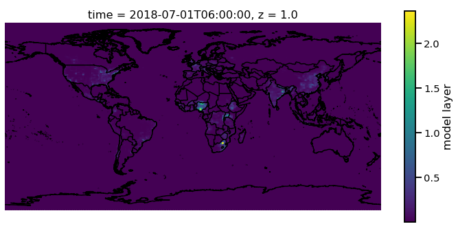
Now one of the main things that will need to be done is plotting on a map. This can be done quickly using the functionality in MONET. In this example we will plot the first layer PM2.5 at time 2018-07-01. Ui
f.pm25[0,0,:,:].monet.quick_map()
[########################################] | 100% Completed |  0.1s
[########################################] | 100% Completed |  0.2s
[########################################] | 100% Completed |  0.1s
[########################################] | 100% Completed |  0.2s
<cartopy.mpl.geoaxes.GeoAxesSubplot at 0x1c164f2dd8>
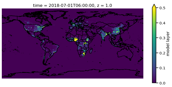
Adjusting the scale is simple by supplying vmin and vmax. Lets
set a minimum of 0 AOD and maximum of 0.5.
f.pm25[0,0,:,:].monet.quick_map(vmin=0,vmax=.5)
[########################################] | 100% Completed |  0.1s
[########################################] | 100% Completed |  0.2s
[########################################] | 100% Completed |  0.1s
[########################################] | 100% Completed |  0.2s
<cartopy.mpl.geoaxes.GeoAxesSubplot at 0x1c18cbf6d8>
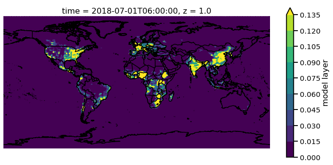
Now we have all the control that xarray has built into their plotting
routines. For example, lets have a discrete colorbar with 10 levels,
levels=10, and let it determine the levels by throwing out the top
and bottom 2% of values using the robust=True
f.pm25[0,0,:,:].monet.quick_map(levels=10,robust=True)
[########################################] | 100% Completed |  0.1s
[########################################] | 100% Completed |  0.2s
[########################################] | 100% Completed |  0.1s
[########################################] | 100% Completed |  0.2s
<cartopy.mpl.geoaxes.GeoAxesSubplot at 0x1c1905ce48>
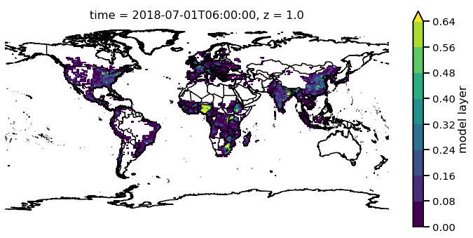
Now there are a lot of very low values, since this is at the beginning of the simulation so lets mask out values less than 0.015 AOD.
f.pm25.where(f.pm25 > 0.015)[0,0,:,:].monet.quick_map(levels=10,robust=True)
[########################################] | 100% Completed |  0.1s
[########################################] | 100% Completed |  0.2s
[########################################] | 100% Completed |  0.1s
[########################################] | 100% Completed |  0.2s
<cartopy.mpl.geoaxes.GeoAxesSubplot at 0x1c19635240>
For more information on plotting with xarray and matplotlib some useful links are shown below
Nearest neighbor
Monet has some extra functionality that may be useful for exploratory studies such as nearest neighbor finder. Lets find the nearest neighbor to NCWCP (38.972 N, 76.9245 W).
nn = f.pm25.monet.nearest_latlon(lat=38.972,lon=-76.9245)
print(nn)
<xarray.DataArray 'pm25' (time: 1, z: 64)>
dask.array<shape=(1, 64), dtype=float32, chunksize=(1, 64)>
Coordinates:
  * time       (time) datetime64[ns] 2018-07-01T06:00:00
    x          float64 283.1
    y          float64 38.81
  * z          (z) float64 1.0 2.0 3.0 4.0 5.0 6.0 ... 60.0 61.0 62.0 63.0 64.0
    longitude  float64 283.1
    latitude   float64 38.81
Attributes:
    long_name:  model layer
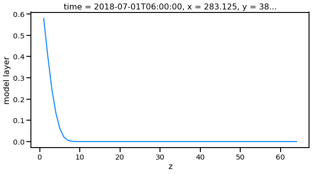
Now we can do a quick plot of this vertically, since it was a single time step.
nn.plot(aspect=2,size=5)
[########################################] | 100% Completed |  0.1s
[########################################] | 100% Completed |  0.1s
[<matplotlib.lines.Line2D at 0x1c194702e8>]
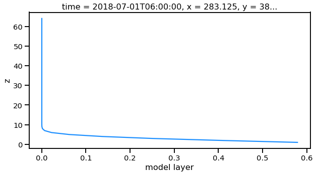
Now this is a simple plot but it is usually valuable to view the vertical coordinate on the y-axis.
nn.plot(y='z',aspect=2,size=5)
[########################################] | 100% Completed |  0.1s
[########################################] | 100% Completed |  0.2s
[########################################] | 100% Completed |  0.1s
[########################################] | 100% Completed |  0.2s
[<matplotlib.lines.Line2D at 0x1c1c0bbac8>]
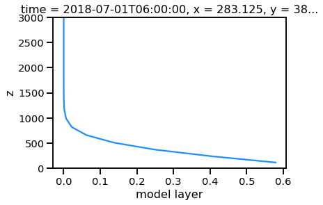
Now this is not very useful because the vertical coordinate right now is just the layer number. Lets get the geopoential height at this location and add it as a coordinate to plot.
geohgt = f.geohgt.monet.nearest_latlon(lat=38.972,lon=-76.9245).squeeze()
geohgt
<xarray.DataArray 'geohgt' (z: 64)>
dask.array<shape=(64,), dtype=float32, chunksize=(64,)>
Coordinates:
    time       datetime64[ns] 2018-07-01T06:00:00
    x          float64 283.1
    y          float64 38.81
  * z          (z) float64 1.0 2.0 3.0 4.0 5.0 6.0 ... 60.0 61.0 62.0 63.0 64.0
    longitude  float64 283.1
    latitude   float64 38.81
Attributes:
    long_name:  Geopotential Height
    units:      m
nn['z'] = geohgt.values
nn.plot(y='z')
plt.ylim([0,3000])
[########################################] | 100% Completed |  0.3s
[########################################] | 100% Completed |  0.4s
[########################################] | 100% Completed |  0.1s
[########################################] | 100% Completed |  0.2s
[########################################] | 100% Completed |  0.1s
[########################################] | 100% Completed |  0.2s
(0, 3000)
Constant Latitude and Longitude
Sometimes it may be useful to see a latitudinal or longitudinal cross
section. This feature is included in monet through the
xr.DataArray.monet accessor. Lets take a constant latitude at 10
degrees N.
pm25_constant_lat = f.pm25.monet.interp_constant_lat(lat=10., method='bilinear')
pm25_constant_lat
Create weight file: bilinear_192x384_192x1.nc
[########################################] | 100% Completed |  0.1s
[########################################] | 100% Completed |  0.2s
<xarray.DataArray 'pm25' (time: 1, z: 64, x: 192, y: 1)>
array([[[[8.107865e-02],
         ...,
         [4.765707e-02]],

        ...,

        [[9.984020e-05],
         ...,
         [9.982444e-05]]]])
Coordinates:
    longitude  (x, y) float64 0.0 1.88 3.76 5.64 ... 353.4 355.3 357.2 359.1
    latitude   (x, y) float64 10.0 10.0 10.0 10.0 10.0 ... 10.0 10.0 10.0 10.0
  * time       (time) datetime64[ns] 2018-07-01T06:00:00
  * z          (z) float64 1.0 2.0 3.0 4.0 5.0 6.0 ... 60.0 61.0 62.0 63.0 64.0
Dimensions without coordinates: x, y
Attributes:
    regrid_method:  bilinear
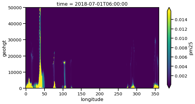
Like before lets go ahead and get the geopotential height along this latitude.
geoght_constant_lat = f.geohgt.monet.interp_constant_lat(lat=10., method='bilinear')
pm25_constant_lat['geohgt'] = geoght_constant_lat
Overwrite existing file: bilinear_192x384_192x1.nc
 You can set reuse_weights=True to save computing time.
[########################################] | 100% Completed |  0.7s
[########################################] | 100% Completed |  0.8s
Let us plot the 2D cross track (height vs longitude).
pm25_constant_lat.plot(x='longitude',y='geohgt',robust=True,ylim=1000,aspect=2,size=5)
plt.ylim([0,50000])
(0, 50000)
Calculate Pressure Levels
By default pressure levels are not calculated due to processing time,
however, MONET does include a helper function in the fv3chem module,
fv3chem.calc_nemsio_pressure.
f = miofv3chem.calc_nemsio_pressure(f)
f
[########################################] | 100% Completed |  0.1s
[########################################] | 100% Completed |  0.2s
[########################################] | 100% Completed |  0.1s
[########################################] | 100% Completed |  0.2s
<xarray.DataArray 'press' (time: 1, z: 64, y: 192, x: 384)>
array([[[[1.002220e+03, ..., 1.002230e+03],
         ...,
         [6.768812e+02, ..., 6.770022e+02]],

        ...,

        [[2.037354e-01, ..., 2.038117e-01],
         ...,
         [3.515549e-01, ..., 3.512193e-01]]]], dtype=float32)
Coordinates:
  * time       (time) datetime64[ns] 2018-07-01T06:00:00
  * x          (x) float64 0.0 0.9375 1.875 2.812 ... 356.2 357.2 358.1 359.1
  * y          (y) float64 89.28 88.36 87.42 86.49 ... -87.42 -88.36 -89.28
  * z          (z) float64 1.0 2.0 3.0 4.0 5.0 6.0 ... 60.0 61.0 62.0 63.0 64.0
    longitude  (y, x) float64 0.0 0.9375 1.875 2.812 ... 356.2 357.2 358.1 359.1
    latitude   (y, x) float64 89.28 89.28 89.28 89.28 ... -89.28 -89.28 -89.28
Attributes:
    units:      mb
    long_name:  Mid Layer Pressure