How to Open and View CMAQ simulations - HI Volcano Example
In this example, we will learn how to open CMAQ simulations using MONET, view the data on a map, view cross sections of the data, and compare to surface observations (AirNow) for the May 2018 Hawaiian volcanic eruption. First, import MONET and several helper functions for later.
import monet as m
import monetio as mio
import matplotlib.pyplot as plt
from monet.util import tools
import pandas as pd
Now the data can be downloaded from the MONET github page in the
MONET/data directory. We will assume you already have this downloaded
and will proceed. Open the simulation. As of right now we still require
that a separate grdcro2d (grddot2d) file be loaded for the mass points
(dot points) using the grid kwarg.
conc = '/Users/barry/Desktop/MONET/data/aqm.t12z.aconc.ncf'
c = mio.cmaq.open_dtaset(flist=conc)
The cmaq object will return a xarray.Dataset but it also still lives
inside of the cmaq object in cmaq.dset. We may use a combination
of both the dataset (c) directly and the cmaq calls to gather or
aggrigate species in the concentration file.
c
<xarray.Dataset>
Dimensions:    (DATE-TIME: 2, VAR: 41, time: 48, x: 80, y: 52, z: 1)
Coordinates:
* time       (time) datetime64[ns] 2018-05-17T12:00:00 2018-05-17T13:00:00 ...
  longitude  (y, x) float64 -161.9 -161.8 -161.7 -161.6 -161.5 -161.4 ...
  latitude   (y, x) float64 17.76 17.76 17.77 17.77 17.77 17.77 17.78 ...
Dimensions without coordinates: DATE-TIME, VAR, x, y, z
Data variables:
  TFLAG      (time, VAR, DATE-TIME) int32 ...
  O3         (time, z, y, x) float32 28.296675 28.461445 28.483536 ...
  NO2        (time, z, y, x) float32 0.0072615896 0.007076008 0.0070880884 ...
  NO         (time, z, y, x) float32 1.6760728e-08 1.6089658e-08 ...
  NO3        (time, z, y, x) float32 0.0022378012 0.0022129775 ...
  N2O5       (time, z, y, x) float32 8.560217e-06 8.241847e-06 ...
  HNO3       (time, z, y, x) float32 0.1326946 0.13388994 0.1343063 ...
  HONO       (time, z, y, x) float32 6.2205704e-06 5.9552485e-06 ...
  PNA        (time, z, y, x) float32 2.1638462e-07 1.9233373e-07 ...
  CO         (time, z, y, x) float32 72.599915 72.56304 72.599266 ...
  FORM       (time, z, y, x) float32 0.3351323 0.3413216 0.34457546 ...
  ALD2       (time, z, y, x) float32 0.13579664 0.12625198 0.1253843 ...
  PAN        (time, z, y, x) float32 0.00054027676 0.00047953427 ...
  NTR        (time, z, y, x) float32 0.0057188044 0.0053887735 0.005364259 ...
  XO2N       (time, z, y, x) float32 2.1813818e-05 2.1018073e-05 ...
  SO2        (time, z, y, x) float32 0.009011468 0.009855208 0.009888159 ...
  ASO4I      (time, z, y, x) float32 0.00071987335 0.0006097436 ...
  ASO4J      (time, z, y, x) float32 0.6792807 0.68186235 0.6739671 ...
  ANH4I      (time, z, y, x) float32 5.4321783e-05 4.6263896e-05 ...
  ANH4J      (time, z, y, x) float32 0.051220056 0.051677197 0.05048342 ...
  ANO3I      (time, z, y, x) float32 9.547329e-16 8.1884126e-16 ...
  ANO3J      (time, z, y, x) float32 8.933346e-13 9.0928e-13 5.418493e-05 ...
  AORGAI     (time, z, y, x) float32 1.4356241e-10 1.308317e-10 ...
  AORGAJ     (time, z, y, x) float32 1.2230534e-05 1.1428401e-05 ...
  AORGPAI    (time, z, y, x) float32 6.7508597e-07 6.614316e-07 ...
  AORGPAJ    (time, z, y, x) float32 0.05786852 0.058112975 0.05817498 ...
  AORGBI     (time, z, y, x) float32 6.7122006e-09 6.5227788e-09 ...
  AORGBJ     (time, z, y, x) float32 0.0005746193 0.00057244353 ...
  AECI       (time, z, y, x) float32 2.4381194e-07 2.3888646e-07 ...
  AECJ       (time, z, y, x) float32 0.014596849 0.014644699 0.014672826 ...
  A25I       (time, z, y, x) float32 ...
  A25J       (time, z, y, x) float32 ...
  NUMATKN    (time, z, y, x) float32 ...
  NUMACC     (time, z, y, x) float32 ...
  SRFATKN    (time, z, y, x) float32 ...
  SRFACC     (time, z, y, x) float32 ...
  AH2OI      (time, z, y, x) float32 ...
  AH2OJ      (time, z, y, x) float32 ...
  ACLI       (time, z, y, x) float32 ...
  ACLJ       (time, z, y, x) float32 3.5000003e-13 3.5000003e-13 ...
  ANAI       (time, z, y, x) float32 8.394818e-17 8.4039525e-17 ...
  ANAJ       (time, z, y, x) float32 0.2311452 0.23135261 0.23287562 ...
  PM25       (time, z, y, x) float32 1.0354732 1.0388906 1.0314605 ...
  PM10       (time, z, y, x) float32 1.0354732 1.0388906 1.0314605 ...
  CLf        (time, z, y, x) float32 3.5000003e-13 3.5000003e-13 ...
  NAf        (time, z, y, x) float32 0.2311452 0.23135261 0.23287562 ...
  NOy        (time, z, y, x) float32 0.0001484681 0.00014906164 ...
  NOx        (time, z, y, x) float32 1.6760728e-11 1.6089657e-11 ...
  NO3f       (time, z, y, x) float32 8.9428936e-13 9.100988e-13 ...
  NH4f       (time, z, y, x) float32 0.051274378 0.05172346 0.050527096 ...
  SO4f       (time, z, y, x) float32 0.68000054 0.6824721 0.67454904 ...
Attributes:
  IOAPI_VERSION:   $Id: @(#) ioapi library version 3.1 $                   ...
  EXEC_ID:         ????????????????                                        ...
  FTYPE:           1
  CDATE:           2018142
  CTIME:           135716
  WDATE:           2018142
  WTIME:           135716
  SDATE:           2018137
  STIME:           120000
  TSTEP:           10000
  NTHIK:           1
  NCOLS:           80
  NROWS:           52
  NLAYS:           1
  NVARS:           41
  GDTYP:           2
  P_ALP:           19.0
  P_BET:           21.0
  P_GAM:           -157.5
  XCENT:           -157.5
  YCENT:           20.53
  XORIG:           -480000.0
  YORIG:           -312000.0
  XCELL:           12000.0
  YCELL:           12000.0
  VGTYP:           1
  VGTOP:           200.0
  VGLVLS:          [1.       0.089794]
  GDNAM:           AQF_HI
  UPNAM:           OPACONC
  VAR-LIST:        O3              NO2             NO              NO3     ...
  FILEDESC:        Concentration file output                               ...
  HISTORY:
  proj4_srs:       +proj=lcc +lat_1=19.0 +lat_2=21.0 +lat_0=20.53 +lon_0=-1...
  area:            Area ID: MONET_Object_GridnDescription: IOAPI area_def ...
  mapping_tables:  {'improve': {}, 'aqs': {'OZONE': ['O3'], 'PM2.5': ['PM25...
Notice that this looks like the ncdump of the file except that there are separate coordinates including the latitude and longitude and the time as numpy.datetime64 objects. Also included is the proj4 string, a pyresample area grid and default mapping tables to several different observational datasets.
Plotting on a map
It is often useful to be able to view the data on a map. Let’s view a random time slice of SO2 (we will view time 20 hours into the simulation). Here will use the MONETAccessor from the MONET package to aid in the plotting.
c.SO2[15,0,:,:].monet.quick_map()
[########################################] | 100% Completed |  0.1s
[########################################] | 100% Completed |  0.1s
[########################################] | 100% Completed |  0.2s
[########################################] | 100% Completed |  0.3s
[########################################] | 100% Completed |  0.3s
[########################################] | 100% Completed |  0.1s
[########################################] | 100% Completed |  0.1s
[########################################] | 100% Completed |  0.2s
[########################################] | 100% Completed |  0.3s
[########################################] | 100% Completed |  0.4s
<matplotlib.collections.QuadMesh at 0x1c27910860>
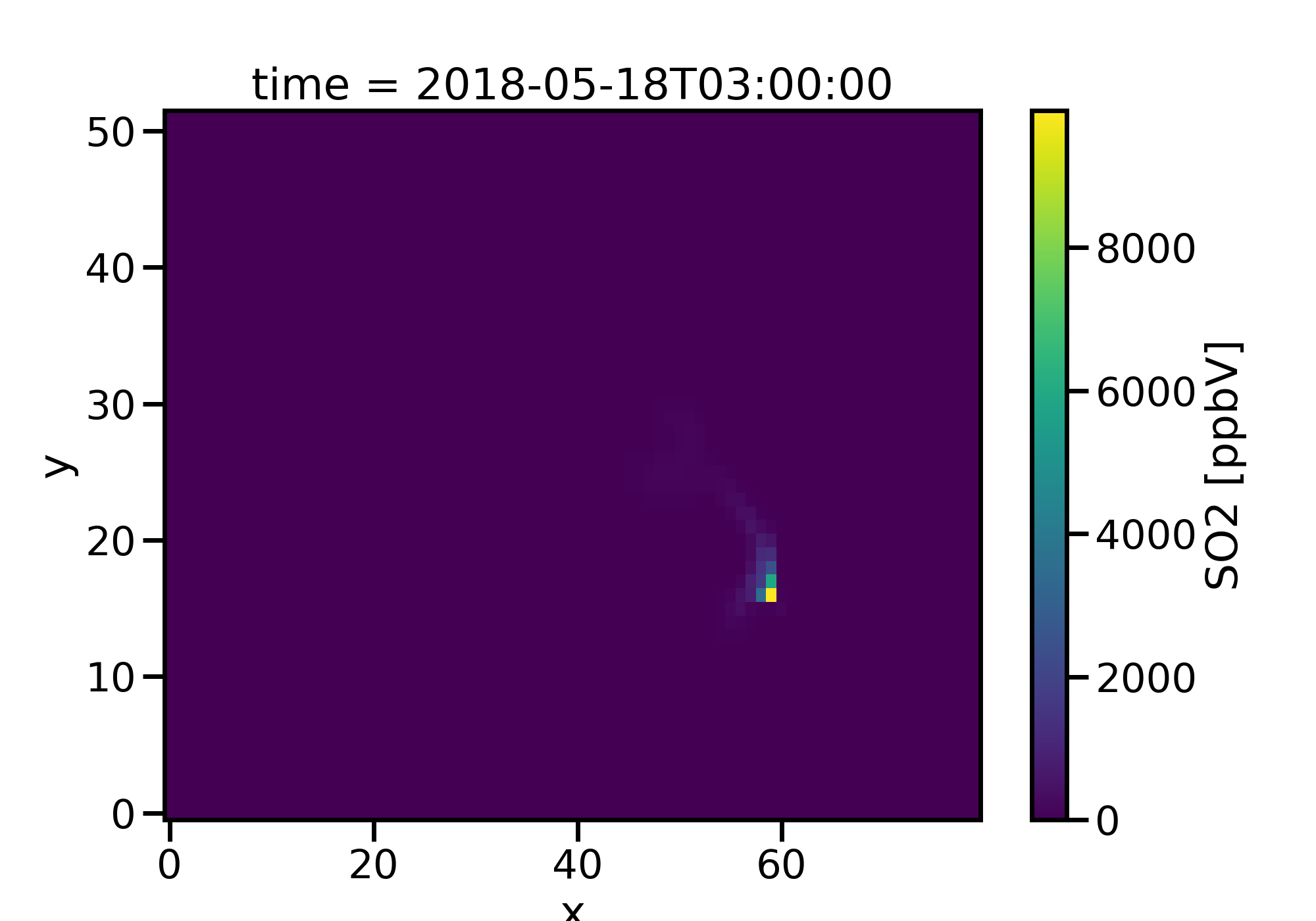
Now this doesn’t look very pretty. First it isn’t on a map, the color
scale isn’t good as we cannot really see any of the data. To fix this we
will add a map using the MONETAccessor and use the robust=True kwarg.
c.SO2[15,0,:,:].monet.quick_map(robust=True)
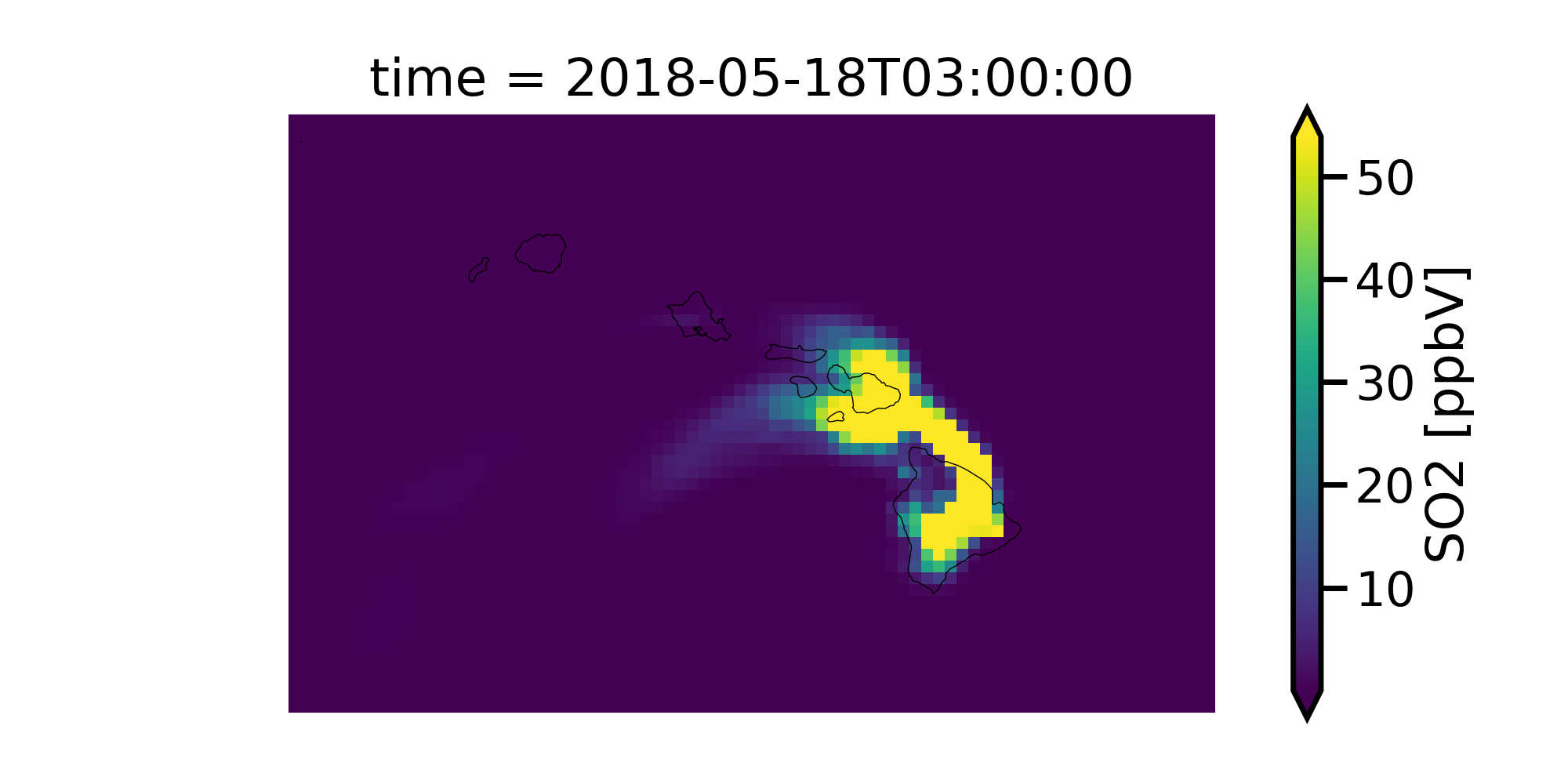
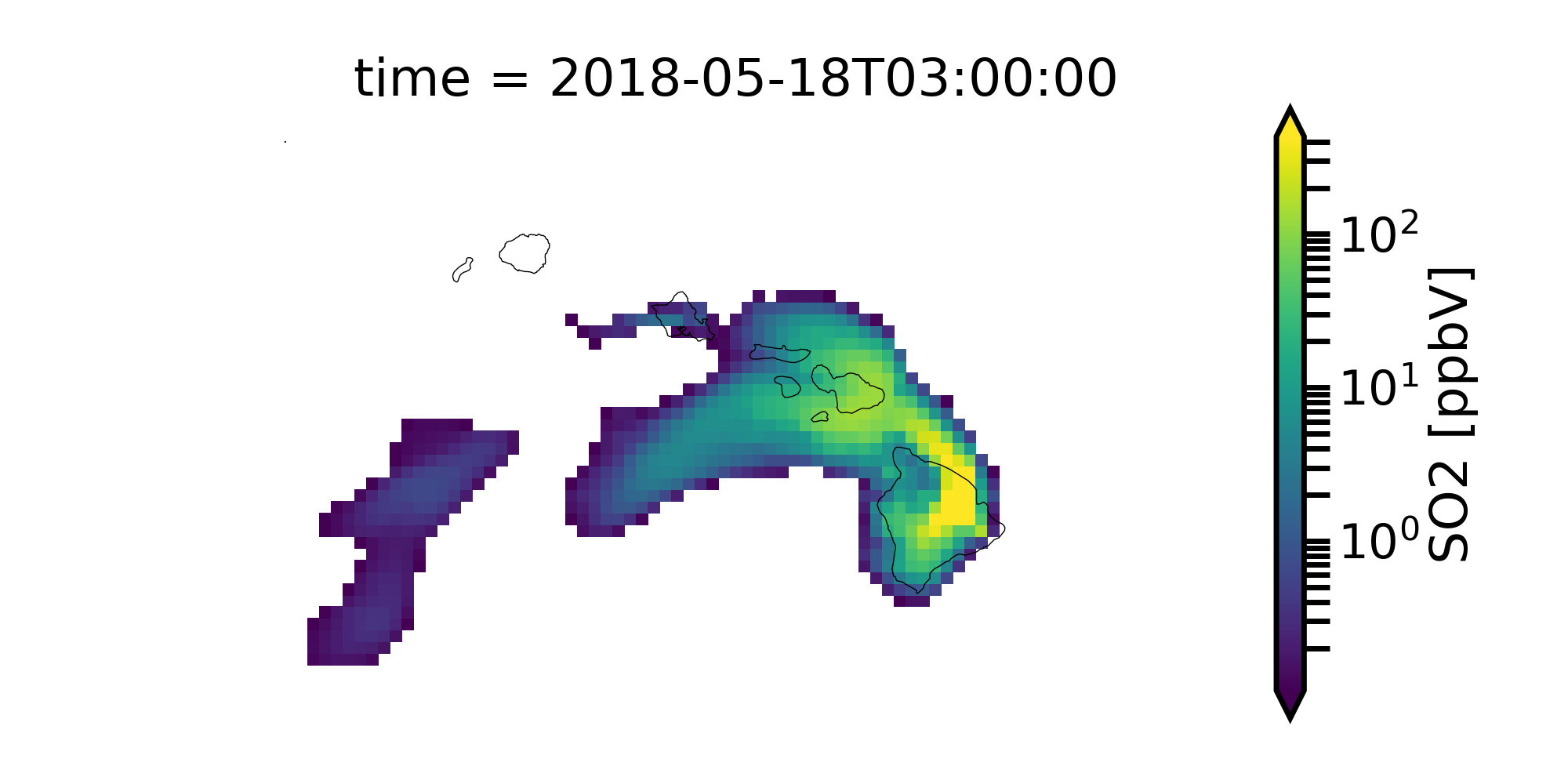
Better but we can still do much more. There is low concentrations on most of this map making it hard to notice the extremely high values and the SO2 data is in ppmv and not ppbv as normally viewed as. Also, a logscale may be better for this type of data as it goes from 0-20000 ppbv rather than a linear scale.
from matplotlib.colors import LogNorm
# convert to ppbv
so2 = c.SO2[15,0,:,:]
so2.where(so2 > 0.1).monet.quick_map(robust=True, norm=LogNorm())
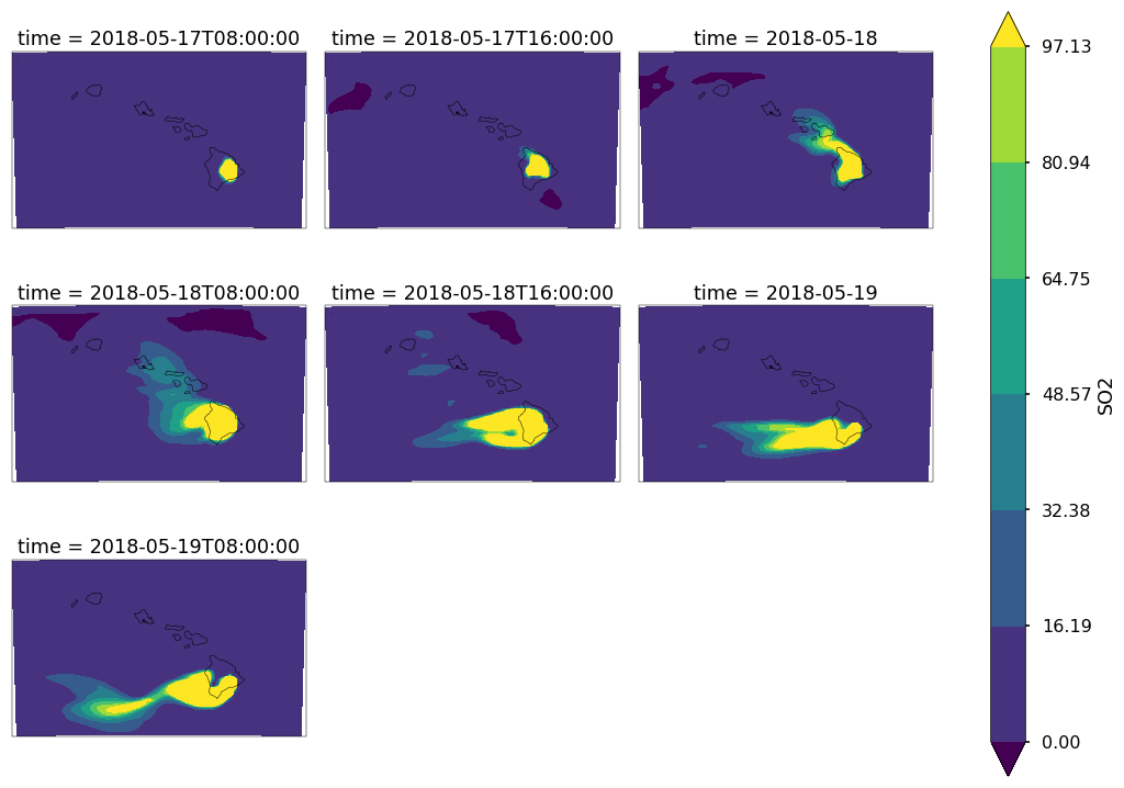
Now let’s us view several time slices at once. We will average in time (every 8 hours) to give us 6 total subplots.
so2 = c.SO2[:,0,:,:] * 1000.
so2_resampled = so2.resample(time='8h').mean('time').sortby(['y', 'x'],ascending=True)
p = so2_resampled.plot.contourf(col_wrap=3,col='time',x='longitude',y='latitude',robust=True,figsize=(15,10),subplot_kws={'projection': ccrs.PlateCarree()})
extent = [so2.longitude.min(),so2.longitude.max(),so2.latitude.min(),so2.latitude.max()]
for ax in p.axes.flat:
    draw_map(ax=ax,resolution='10m',extent=extent)
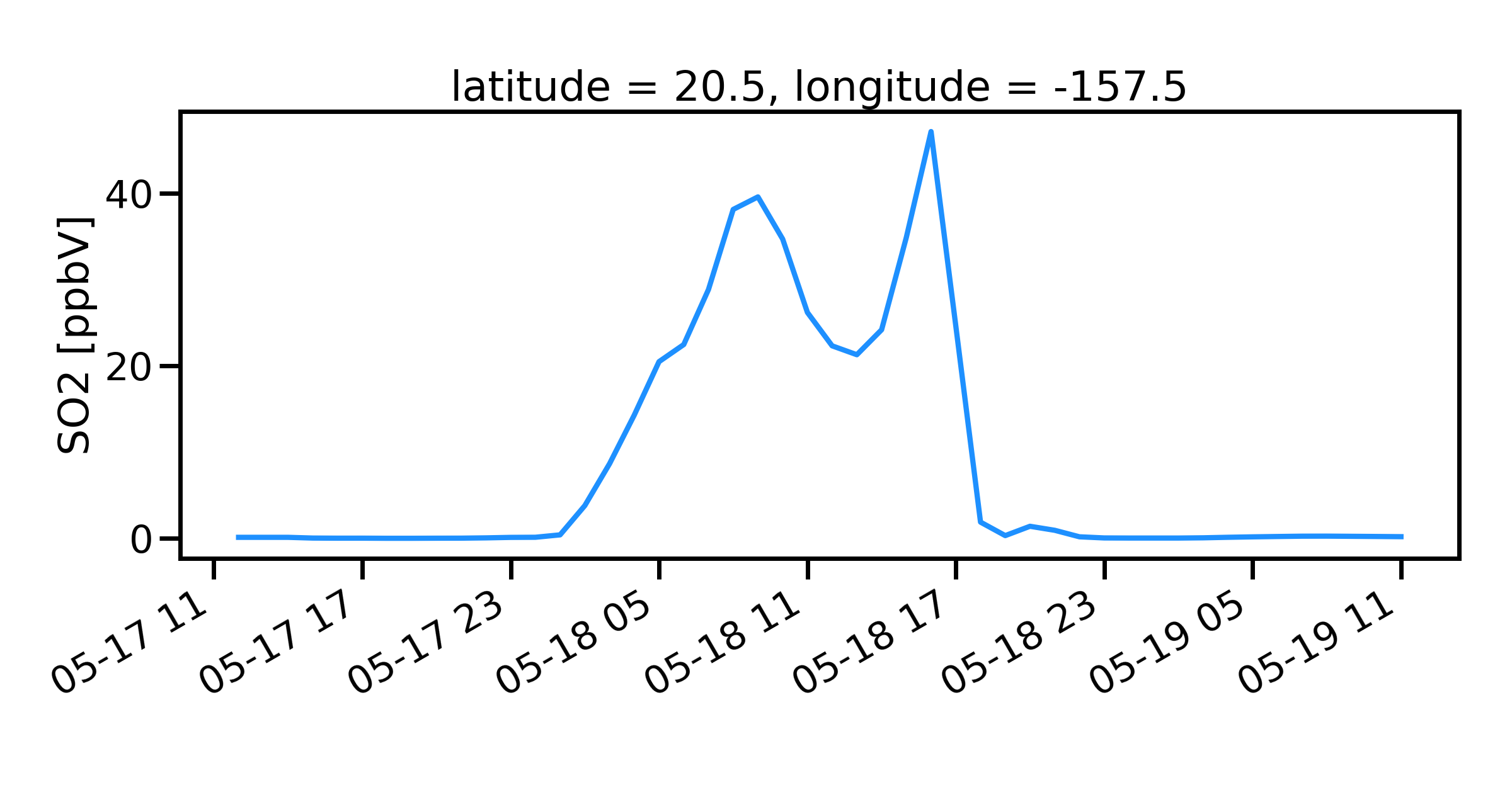
Finding nearest lat lon point
Suppose that we want to find the model data found at a point (latitude,longitude). Use the MONETAccessor again
so2.monet.nearest_latlon(lat=20.5,lon=157.5).plot(figsize=(12,6))
plt.xlabel('')
plt.tight_layout()
Pairing with AirNow
It is often useful to be able to pair model data with observational data. MONET uses the pyresample library (http://pyresample.readthedocs.io/en/latest/) to do a nearest neighbor interpolation. First let us get the airnow data for the dates of the simulation. We will also rotate it from the raw AirNow long format (stacked variables) to a wide format (each variable is a separate column)
df = mio.airnow.add_data(so2.time.to_index())
Aggregating AIRNOW files...
Building AIRNOW URLs...
[########################################] | 100% Completed |  1.3s
[########################################] | 100% Completed |  1.4s
[########################################] | 100% Completed |  1.4s
[########################################] | 100% Completed |  1.5s
[########################################] | 100% Completed |  1.5s
[########################################] | 100% Completed | 12.3s
[########################################] | 100% Completed | 12.4s
[########################################] | 100% Completed | 12.4s
[########################################] | 100% Completed | 12.5s
[########################################] | 100% Completed | 12.6s
    Adding in Meta-data
Now let us combine the two. This will return the pandas dataframe with a new column (model).
df_combined = so2.monet.combine_point(df,col='SO2')
[########################################] | 100% Completed |  0.1s
[########################################] | 100% Completed |  0.2s
[########################################] | 100% Completed |  0.1s
[########################################] | 100% Completed |  0.2s
[########################################] | 100% Completed |  0.1s
[########################################] | 100% Completed |  0.2s
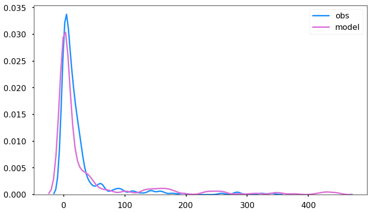
Let’s look at the distributions to see if the two overlap to get a general sense of performance.
df_so2 = df.loc[(df.variable == 'SO2') & (df.state_name == 'HI')].dropna(subset=['obs'])
import seaborn as sns
f,ax = plt.subplots(figsize=(12,7))
sns.kdeplot(df_so2.obs, ax=ax, clip=[0,500])
sns.kdeplot(df_so2.model,ax=ax, clip=[0,500])
<matplotlib.axes._subplots.AxesSubplot at 0x1c290e94a8>
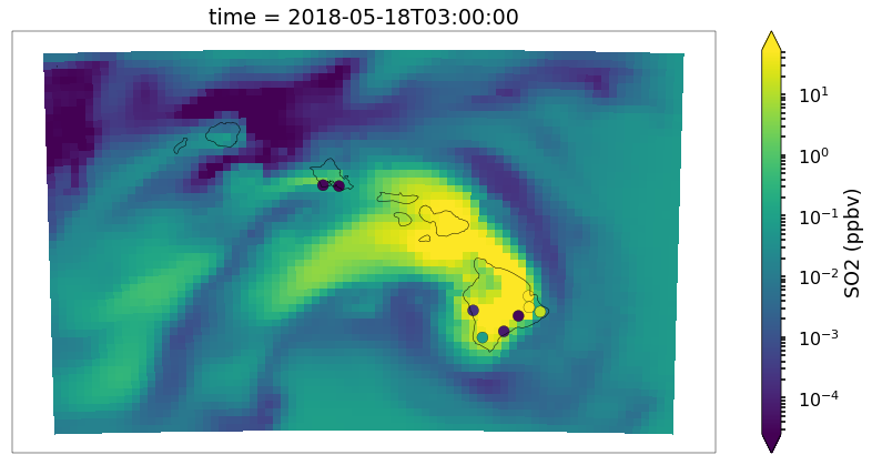
Overlaying Observations on Contour Plots
Now let’s put a time slice on a map. Let’s look back to the time step ‘2018-05-18 03:00’,
from monet.plots import *
ax = draw_map(states=True, resolution='10m', figsize=(15,7))
so2_now = so2.sel(time='2018-05-18 03:00')
p = so2_now.plot(x='longitude',y='latitude',ax=ax, robust=True,norm=LogNorm(),cbar_kwargs={'label': 'SO2 (ppbv)'})
vmin,vmax = p.get_clim()
cmap = p.get_cmap()
d = df_so2.loc[df_so2.time == '2018-05-18 03:00']
plt.scatter(d.longitude.values,d.latitude.values,c=d.obs,cmap=cmap,vmin=vmin,vmax=vmax)
{'figsize': (15, 7), 'subplot_kw': {'projection': <cartopy.crs.PlateCarree object at 0x1c27451d00>}}
[########################################] | 100% Completed |  0.1s
[########################################] | 100% Completed |  0.2s
[########################################] | 100% Completed |  0.3s
[########################################] | 100% Completed |  0.3s
[########################################] | 100% Completed |  0.4s
<matplotlib.collections.PathCollection at 0x1c2ae207b8>

Not bad but again we can do a little better with the scatter plot. It’s hard to see the outlines of the observations when there is high correlation, the sizes may be a little large
ax = draw_map(states=True, resolution='10m', figsize=(15,7))

so2_now = so2.sel(time='2018-05-18 03:00')
p = so2_now.plot(x='longitude',y='latitude',ax=ax, robust=True,norm=LogNorm(),cbar_kwargs={'label': 'SO2 (ppbv)'})
vmin,vmax = p.get_clim()
cmap = p.get_cmap()
d = df_so2.loc[df_so2.time == '2018-05-18 03:00']
plt.scatter(d.longitude.values,d.latitude.values,c=d.obs,cmap=cmap,s=100,edgecolors='k',lw=.25, vmin=vmin,vmax=vmax)
{'figsize': (15, 7), 'subplot_kw': {'projection': <cartopy.crs.PlateCarree object at 0x1c2b0ead00>}}
[########################################] | 100% Completed |  0.1s
[########################################] | 100% Completed |  0.1s
[########################################] | 100% Completed |  0.1s
[########################################] | 100% Completed |  0.2s
[########################################] | 100% Completed |  0.3s
[########################################] | 100% Completed |  0.1s
[########################################] | 100% Completed |  0.2s
[########################################] | 100% Completed |  0.3s
[########################################] | 100% Completed |  0.4s
[########################################] | 100% Completed |  0.5s
<matplotlib.collections.PathCollection at 0x1c2b43c5f8>
p = df_so2.loc[df_so2.obs > 10]
p.obs.std()
61.45120441800254