NOAA NESDIS AOD
NOAA NESDIS has an operational data product for the aerosol optical depth from the VIIRS satellite. There are two products, the viirs edr and viirs eps available from ftp://ftp.star.nesdis.noaa.gov/pub/smcd/.
VIIRS EDR
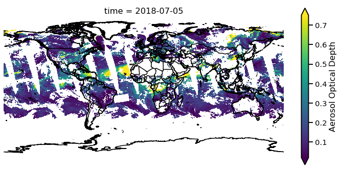
The VIIRS EDR data is an aerosol optical depth product available at 0.1 and 0.25 degree resolution. This VIIRS EDR product also does not include the Blue Sky algorithm to retrieve over bright surfaces such as the Sahara. Lets open the data on a single day at first, in this case ‘2018-07-05’.
import monetio as mio
edr = mio.nesdis_edr_viirs.open_dataset('2018-07-05')
print(edr)
<xarray.DataArray 'VIIRS EDR AOD' (time: 1, y: 1800, x: 3600)>
array([[[nan, nan, ..., nan, nan],
        [nan, nan, ..., nan, nan],
        ...,
        [nan, nan, ..., nan, nan],
        [nan, nan, ..., nan, nan]]], dtype=float32)
Coordinates:
  * time       (time) datetime64[ns] 2018-07-05
  * y          (y) int64 0 1 2 3 4 5 6 7 ... 1793 1794 1795 1796 1797 1798 1799
  * x          (x) int64 0 1 2 3 4 5 6 7 ... 3593 3594 3595 3596 3597 3598 3599
    latitude   (y, x) float64 -89.88 -89.88 -89.88 -89.88 ... 89.88 89.88 89.88
    longitude  (y, x) float64 -179.9 -179.8 -179.7 -179.6 ... 179.7 179.8 179.9
Attributes:
    units:
    long_name:  Aerosol Optical Depth
    source:     ftp://ftp.star.nesdis.noaa.gov/pub/smcd/jhuang/npp.viirs.aero...
edr is now a xarray.DataArray for that day. The
nesdis_edr_viirs module downloads data to the current directory. To
download this into a different directory you can supply the
datapath= keyword if needed. To quickly view this you can use the
monet accessor.
edr.monet.quick_map(robust=True)
<cartopy.mpl.geoaxes.GeoAxesSubplot at 0x1022a77470>
The EDR data is available in two resolutions. By default monet will
download the 0.1 degree dataset. If you would like the 0.25 degree
dataset you can pass the kwarg resolution='low'.
edr = mio.nesdis_edr_viirs.open_dataset('2018-07-05', resolution='low')
print(edr)
<xarray.DataArray 'VIIRS EDR AOD' (time: 1, y: 720, x: 1440)>
array([[[nan, nan, ..., nan, nan],
        [nan, nan, ..., nan, nan],
        ...,
        [nan, nan, ..., nan, nan],
        [nan, nan, ..., nan, nan]]], dtype=float32)
Coordinates:
  * time       (time) datetime64[ns] 2018-07-05
  * y          (y) int64 0 1 2 3 4 5 6 7 8 ... 712 713 714 715 716 717 718 719
  * x          (x) int64 0 1 2 3 4 5 6 7 ... 1433 1434 1435 1436 1437 1438 1439
    latitude   (y, x) float64 -89.88 -89.88 -89.88 -89.88 ... 89.88 89.88 89.88
    longitude  (y, x) float64 -179.9 -179.6 -179.4 -179.1 ... 179.4 179.6 179.9
Attributes:
    units:
    long_name:  Aerosol Optical Depth
    source:     ftp://ftp.star.nesdis.noaa.gov/pub/smcd/jhuang/npp.viirs.aero...
Notice that the dimensions changed from 1800x3600 to 720x1440.
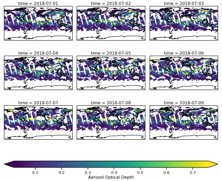
Open Multiple Days
If you want to open multiple days in a single call you could use the open_mfdataset. Lets grab the first nine days of July 2018.
import pandas as pd
dates = pd.date_range(start='2018-07-01',end='2018-07-09')
edr = mio.nesdis_edr_viirs.open_mfdataset(dates)
print(edr)
<xarray.DataArray 'VIIRS EDR AOD' (time: 9, y: 1800, x: 3600)>
array([[[nan, nan, ..., nan, nan],
        [nan, nan, ..., nan, nan],
        ...,
        [nan, nan, ..., nan, nan],
        [nan, nan, ..., nan, nan]],

       [[nan, nan, ..., nan, nan],
        [nan, nan, ..., nan, nan],
        ...,
        [nan, nan, ..., nan, nan],
        [nan, nan, ..., nan, nan]],

       ...,

       [[nan, nan, ..., nan, nan],
        [nan, nan, ..., nan, nan],
        ...,
        [nan, nan, ..., nan, nan],
        [nan, nan, ..., nan, nan]],

       [[nan, nan, ..., nan, nan],
        [nan, nan, ..., nan, nan],
        ...,
        [nan, nan, ..., nan, nan],
        [nan, nan, ..., nan, nan]]], dtype=float32)
Coordinates:
  * y          (y) int64 0 1 2 3 4 5 6 7 ... 1793 1794 1795 1796 1797 1798 1799
  * x          (x) int64 0 1 2 3 4 5 6 7 ... 3593 3594 3595 3596 3597 3598 3599
    latitude   (y, x) float64 -89.88 -89.88 -89.88 -89.88 ... 89.88 89.88 89.88
    longitude  (y, x) float64 -179.9 -179.8 -179.7 -179.6 ... 179.7 179.8 179.9
  * time       (time) datetime64[ns] 2018-07-01 2018-07-02 ... 2018-07-09
Attributes:
    units:
    long_name:  Aerosol Optical Depth
    source:     ftp://ftp.star.nesdis.noaa.gov/pub/smcd/jhuang/npp.viirs.aero...
We can visualize these in a seaborn FacetGrid through xarray. For more
information on FacetGrid in xarray plotting please look here:
https://xarray.pydata.org/en/stable/user-guide/plotting.html#faceting
import cartopy.crs as ccrs # map projections and coastlines
cbar_kwargs=dict(orientation='horizontal',pad=0.1, aspect=30)
d = mio.edr.plot.pcolormesh(x='longitude',y='latitude',col='time',col_wrap=3,
                        figsize=(12,12),robust=True,cbar_kwargs=cbar_kwargs,
                       subplot_kws={'projection':ccrs.PlateCarree()})
for ax in d.axes.flat:
    ax.coastlines()
VIIRS EPS
The VIIRS EPS data includes the Blue Sky algorithm in the AOD
calculation. The same methods are available as with the
nesdis_edr_viirs methods.
eps = mio.nesdis_eps_viirs.open_dataset('2018-07-05')
print(eps)
<xarray.DataArray 'VIIRS EPS AOT' (time: 1, y: 720, x: 1440)>
array([[[nan, nan, ..., nan, nan],
        [nan, nan, ..., nan, nan],
        ...,
        [nan, nan, ..., nan, nan],
        [nan, nan, ..., nan, nan]]], dtype=float32)
Coordinates:
    latitude   (y, x) float64 89.88 89.88 89.88 89.88 ... -89.88 -89.88 -89.88
    longitude  (y, x) float64 -179.9 -179.6 -179.4 -179.1 ... 179.4 179.6 179.9
  * time       (time) datetime64[ns] 2018-07-05
Dimensions without coordinates: y, x
Attributes:
    units:
    long_name:  Aerosol Optical Thickness
    source:     ftp://ftp.star.nesdis.noaa.gov/pub/smcd/VIIRS_Aerosol/npp.vii...
eps.monet.quick_map(robust=True)
<cartopy.mpl.geoaxes.GeoAxesSubplot at 0x1c3406d080>
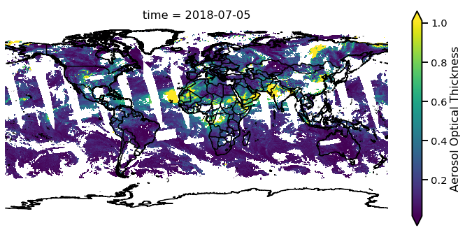
Notice that there are AOD values over deserts such as the Sahara, Australia, northern China, Mongolia and the Middle East